Expectation Maximization algorithm
Published:
I. Expectation Maximization
Expectation Maximization algorithm is widly used in latent variable setting such as semi-supervised, weakly supervised deep learning. We need to understand the EM algorithm before working on this kind of semi- and weakly- supervised settings in deep learning (check ). I present here a intuitive example (basing on a short explanation in this notebook):
1. Setup
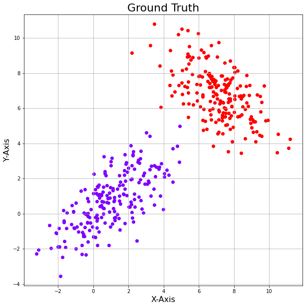
Suppose we have two sets of data points which are two different Gaussian distributions but we dont know which points belonging to which distribution. We will use the EM algorithm to cluster the data points into 2 cluster, corresponding to two Gaussian model and to find these two models parameters (2 components of the Gaussian Mixture Model).
%matplotlib inline
import numpy as np
import matplotlib.cm as cm
import matplotlib.pyplot as plt
import random
from scipy.stats import multivariate_normal     # for generating pdf
np.random.seed(110) # for reproducible results
random.seed(1010) # for reproducible results

m1 = [1,1]      # consider a random mean and covariance value
m2 = [7,7]
cov1 = [[3, 2], [2, 3]]
cov2 = [[2, -1], [-1, 2]]
x = np.random.multivariate_normal(m1, cov1, size=(200,))  # Generating 200 samples for each mean and covariance
y = np.random.multivariate_normal(m2, cov2, size=(200,))
data = np.concatenate((x, y), axis=0)

def plotData(data):
    plt.figure(figsize=(10,10))
    colors = cm.rainbow(np.linspace(0, 1, len(data)))
    for d, c in zip(data, colors):
        plt.scatter(d[:,0], d[:,1], color=c, marker='o')
#     plt.scatter(data[:,0], data[:,1], marker='o')
    plt.axis('equal')
    plt.xlabel('X-Axis', fontsize=16)
    plt.ylabel('Y-Axis', fontsize=16)
    plt.title('Ground Truth', fontsize=22)
    plt.grid()
    plt.show()
plotData([x,y])

2. Expectation Maximization algorithm
The Expectation Maximization algorithm is described as follows:
- We make initial guess (random) of the parameters of 2 components Gaussian mixture model (mean, covariance matrix and mixture probabilities $p_1$ and $p2$).
- EStep: Using the current model paramters, we estimate the likelihood that each point is drawn from a model (using the probability density function). Then we compute the weight that each point belongs to a distribution.
- MStep: Using the estimated probabilities, we update the parameters of the GMM to maximize the likelihood
- Repeat EStep-MStep until the parameters have converged, or a number of iterations has been reached.
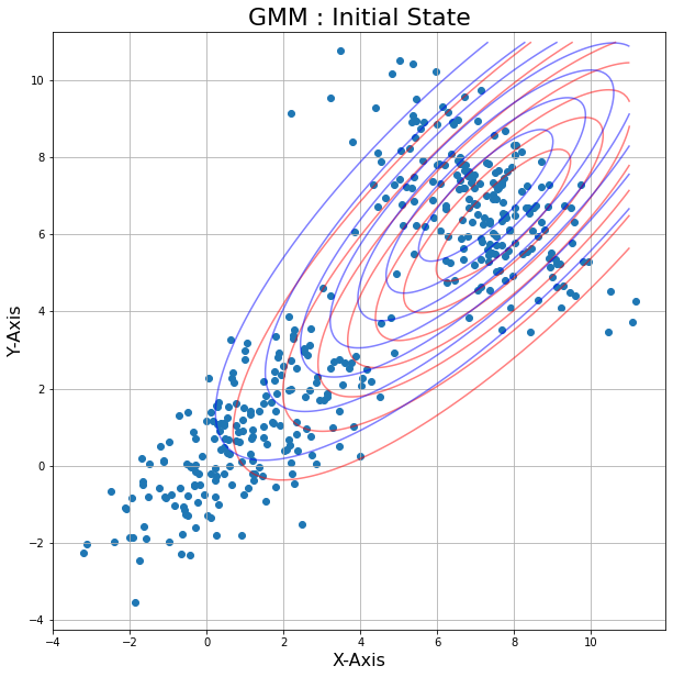
We make initial guess (random) of the GMM.
m1 = random.choice(data)
m2 = random.choice(data)
cov1 = np.cov(np.transpose(data))
cov2 = np.cov(np.transpose(data))
p1 = 0.5
p2 = 1-p1
#Probability density function of 2 Gaussian distributions : Initial State
def plotPDF(m1,m2,cov1,cov2, data):
    x1 = np.linspace(-4,11,200)
    x2 = np.linspace(-4,11,200)
    X, Y = np.meshgrid(x1,x2)

    Z1 = multivariate_normal(m1, cov1)
    Z2 = multivariate_normal(m2, cov2)

    pos = np.empty(X.shape + (2,))                # a new array of given shape and type, without initializing entries
    pos[:, :, 0] = X; pos[:, :, 1] = Y
    print (pos.shape)
    plt.figure(figsize=(10,10))                                                          # creating the figure and assigning the size
    plt.scatter(data[:,0], data[:,1], marker='o')
    plt.contour(X, Y, Z1.pdf(pos), colors="r" ,alpha = 0.5)
    plt.contour(X, Y, Z2.pdf(pos), colors="b" ,alpha = 0.5)
    plt.axis('equal')                                                                  # making both the axis equal
    plt.xlabel('X-Axis', fontsize=16)                                                  # X-Axis
    plt.ylabel('Y-Axis', fontsize=16)                                                  # Y-Axis
    plt.title('GMM : Initial State', fontsize=22)                                            # Title of the plot
    plt.grid()                                                                         # displaying gridlines
    plt.show()

plotPDF(m1,m2,cov1,cov2, data)

The function below is used to compute the weight from the likelihood of each points for each group
def groupWeight(group_likelihood, total_likelihood):
    """
    Compute the weight for each group at each data point.
    group_likelihood is a vector of the likelihood (w.r.t a group) for all points
    total_likelihood is a vector of the sum of the likelihood of each point (w.r.t two groups)
    """
    return group_likelihood / total_likelihood
The two functions below describe the Expectation step and Maximization step. (Loop over data points instead of matrix multiplication for easy understanding)
def Estep(data, m1,m2,cov1,cov2, p1):
    """
    Expectation step : compute the likelihood of each data points for each distribution
    m1,m2,cov1,cov2 is the current parameters of the two Gaussian models
    """
    pt2 = multivariate_normal.pdf(data, mean=m2, cov=cov2)
    pt1 = multivariate_normal.pdf(data, mean=m1, cov=cov1)
    total = p1*pt1+(1-p1)*pt2
    return groupWeight(pt1,total), groupWeight(pt2,total), np.sum(groupWeight(pt1,total))/len(data)

def Mstep(data, weight1, weight2):
    """
    Maximization step : maximize the likelihood of each data points
    """
    num_mu1,din_mu1,num_mu2,din_mu2=0,0,0,0

    for i in range(0,len(data)):
        num_mu1 += weight1[i] * data[i]
        din_mu1 += weight1[i]

        num_mu2 += weight2[i] * data[i]
        din_mu2 += weight2[i]

    mu1 = num_mu1/din_mu1
    mu2 = num_mu2/din_mu2

    num_s1,din_s1,num_s2,din_s2=0,0,0,0
    for i in range(0,len(data)):

        q1 = np.matrix(data[i]-mu1)
        num_s1 += pt1[i] * np.dot(q1.T, q1)
        din_s1 += pt1[i]

        q2 = np.matrix(data[i]-mu2)
        num_s2 += pt2[i] * np.dot(q2.T, q2)
        din_s2 += pt2[i]

    s1 = num_s1/din_s1
    s2 = num_s2/din_s2

    return mu1,mu2,s1,s2
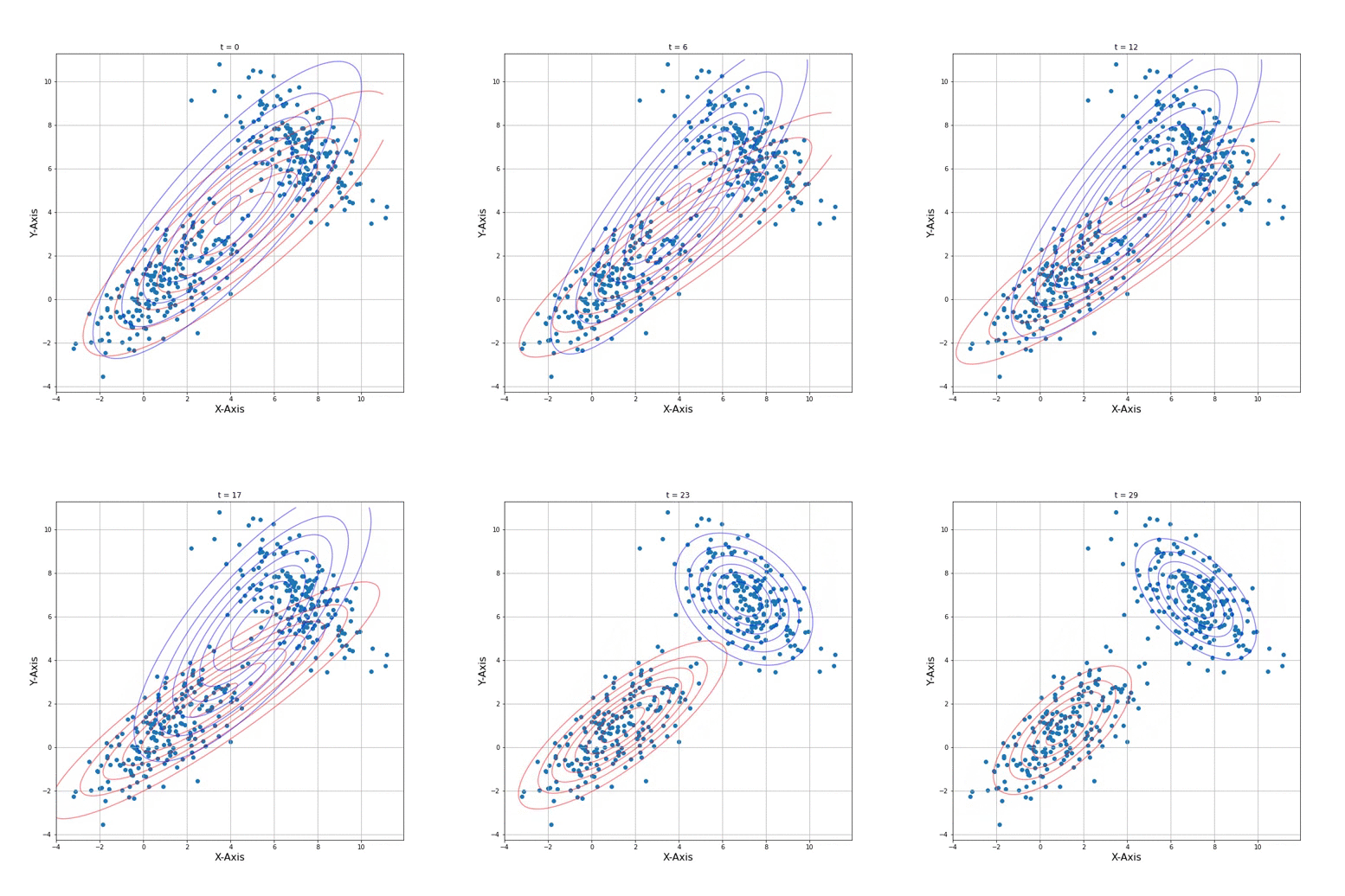
3. Run EM algorithm and draw the animation
def animate(i):
    """
    Repeat EStep and MStep : we put the iteration process in this function because
    we need the save the animation.
    """
    global m1,m2,cov1,cov2,p1
    global cont1, cont2
    #Estimate the GMM model
    pt1, pt2, p1 = Estep(data, m1,m2,cov1,cov2, p1)
    #Maximize the likelihood using current estimated GMM model
    m1,m2,cov1,cov2 = Mstep(data, pt1, pt2)

    #the two Gaussian components
    Z1 = multivariate_normal(m1, cov1)
    Z2 = multivariate_normal(m2, cov2)

    # We nee clear the drawing from previous iterations
    if cont1 is not None:
        for c in cont1.collections:
            c.remove()  # removes only the contours, leaves the rest intact
    if cont2 is not None:
        for c in cont2.collections:
            c.remove()  # removes only the contours, leaves the rest intact

    #Plot the GMM model
    cont1 = plt.contour(X, Y, Z1.pdf(pos), colors="r" ,alpha = 0.5)
    cont2 = plt.contour(X, Y, Z2.pdf(pos), colors="b" ,alpha = 0.5)
    plt.title(r't = %i' % i)
    return cont1, cont2


import matplotlib.animation as animation
# Set up formatting for the movie files
Writer = animation.writers['ffmpeg']
writer = Writer(fps=15, metadata=dict(artist='Me'), bitrate=1800)

cmap = plt.get_cmap('jet')
iterations = 60
pi = 0.7
ims = []
fig = plt.figure(figsize=(10,10))
plt.axis('equal')             # making both the axis equal
plt.scatter(data[:,0], data[:,1], marker='o')
plt.xlabel('X-Axis', fontsize=16)                                                  # X-Axis
plt.ylabel('Y-Axis', fontsize=16)                                                  # Y-Axis
plt.grid()
x1 = np.linspace(-4,11,200)
x2 = np.linspace(-4,11,200)
X, Y = np.meshgrid(x1,x2)
pos = np.empty(X.shape + (2,))                # a new array of given shape and type, without initializing entries
pos[:, :, 0] = X; pos[:, :, 1] = Y

cont1, cont2 = None, None
anim = animation.FuncAnimation(fig, animate, interval=300, frames=iterations)
anim.save('animation.mp4')
